
Have you ever felt your phone hears your conversation? For example, you and your friend are talking about new shoes, and then when you pick your phone up, you get a bunch of ads about it? Or, when you watch a movie or series on Netflix, the next time you get recommendations of your taste? Well, this all is possible thanks to Machine Learning! If you have not heard about it, let me explain it to you. Machine Learning is a very popular topic nowadays. It is a method to analyze data in analytical performance. Machine Learning helps humans with very complicated topics, such as forecasting bitcoin price. In machine learning, the AI model learns from data, analyzes it, and, then, establishes patterns to make future decisions.
Have you ever felt your phone hears your conversation? For example, you and your friend are talking about new shoes, and then when you pick your phone up, you get a bunch of ads about it? Or, when you watch a movie or series on Netflix, the next time you get recommendations of your taste? Well, this all is possible thanks to Machine Learning! If you have not heard about it, let me explain it to you. Machine Learning is a very popular topic nowadays. It is a method to analyze data in analytical performance. Machine Learning helps humans with very complicated topics, such as forecasting bitcoin price. In machine learning, the AI model learns from data, analyzes it, and, then, establishes patterns to make future decisions.
In this and in the following tutorials, you will learn the basics of Machine Learning using Python. In this tutorial, linear regression will be explained. Before we start coding, what is linear regression? Well, linear regression is an algorithm where the predicted values have a linear slope. In general, regression is mostly used to find the relationship between the variables and forecasting. In the case of linear regression, this relationship will be linear.
In this tutorial, the linear regression will be made using matrix multiplication. If we remember our high school Math lessons, a linear relationship between the dependent and independent variables has the form: \[y = c_{0}*x^{0} + c_{1}*x^{1}\] or \[y = c_{0} + c_{1}*x\], where $c_0$ is the intercept with the y-axis, and $c_1$ - the slope of the line.
This relationship can be expressed in a matrix way. In the system, we will have 3 matrices. The first one will be the values of $y$, the second one will be a set of $x$ (in this case we will have only $x_0$ and $x_1$) known as Vandermonde matrix, and the third matrix will consist of the coefficients of $x$
Said this, let's start coding! For this tutorial, the y- and x-values are in a text file named 'points.txt' saved in the same directory as your Python file, The first thing we should do is to import the x- and y- values from the text file into Python. As you already learned previously, data can be imported into a DataFrame using the pandas library (please go to Python: Pandas DataFrame data manipulation). However, in this case, we will import the data into an array using the numpy library.
#Importing library
import numpy as np


#Importing text file
data = np.loadtxt('points.txt', skiprows=(2), dtype=float)
print(data)
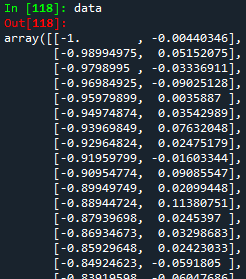
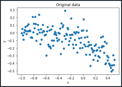
The picture above shows a small part of the whole data. As you can notice, it is a 2D-array where the x- and y-values are delimited by the comma (right and left respectively). To have an idea how these data look like, let's first set our x- and y-values and then, plot them. For this, we will use the matplotlib.pyplot library.
#Importing libraries
import matplotlib.pyplot as plt


#Setting x- and y- values
x = data[:,0]
y = data[:,1]


#Plotting data
plt.plot(x,y,'o')
plt.title('Original data')
plt.xlabel('x')
plt.ylabel('y')
plt.show()
Now, let's define our Vandermonde matrix. In linear algebra, a Vandermonde matrix is a matrix with terms of a geometric progression in each row:
\begin{bmatrix} x_1^0 & x_1^1 & x_1^2 & x_1^3 & ... & x_1^4\\ x_2^0 & x_2^1 & x_2^2 & x_2^3 & ... & x_2^4\\ x_3^0 & x_3^1 & x_3^2 & x_3^3 & ... & x_3^4\\ ... & ... & ... & ... & ... & ...\\ x_n^0 & x_n^1 & x_n^2 & x_n^3 & ... & x_n^4 \end{bmatrix} Notice that d stands for the degree of the polynomial, and n stands for the number of x-values. In this case, since we have a linear relationship, our Vandermonde matrix will be:
Please note that the Vandermonde matrix has dimensions $nx2$ ($n$ rows and 2 columns). In Python, we will build it in the following way:
#Vandermonde matrix
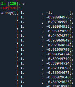
v = np.vstack((np.ones(len(x)),x)).T
print(v)
How to understand the code above? Well, first we create the column-vector of 1s. Remember that the number of 1s in that column is the same as the x-values. To do so, we use the function np.ones. Then, the second column is exactly as the already defined x-array. Finally, the function np.vstack is used to join these two arrays into one.
But, be careful! After doing this, we will get a matrix of $2xn$ (2 rows and $n$ columns). To make this matrix have a dimension $nx2$, we should transpose it. In Python, this is done using .T function. If we run the code above, we will get the Vandermonde matrix.
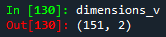
To check the dimensions of the array, we use the function shape.
#Checking dimensions
dimensions_v = v.shape
print(dimensions_v)
Now, it is time to find our coefficients! Like for $x$, we will express the coefficients as a matrix. To do so, let's remember a bit of linear algebra. Since the goal is to minimize the mean square error of the system, the coefficient matrix will be defined as:
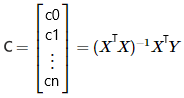
Let's write the above formula in Python.
#Defining the coefficient matrix
coeff = np.linalg.inv(v.T.dot(v)).dot(v.T).dot(y)
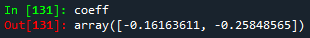
In Python, the inverse of a matrix is written using the function np.linalg.inv(), and in order to multiply matrices, it is necessary to use the function .dot(), otherwise, if you type the common symbol for multiplication '*', you will get an error. If we print the variable coeff, we will get an array consisting of all the coefficients (in this case only $c_0$ and $c_1$)
#Printing the coefficient matrix
print(coeff)
The final step is to build the linear relationship. For this, we will just write the formula which describes this relationship.
#Setting the linear relationship
y_lineal = v.dot(coeff)
print(y_lineal)
In order to know how the straight line through all the initially given x- and y- values looks like, let's plot.
#Plotting


#Initially given x- and y-points
plt.scatter(x,y)


#Linear regression points
plt.plot(x, y_lineal, color='red')


#Naming the graph, x- and y-axis
plt.title('Matrix multiplication')
plt.xlabel('x')
plt.ylabel('y')
plt.show()
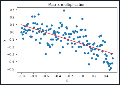
Notice that the blue points are the initially given x- and y-values and the red line is the linear regression model we just built.
The final Python code will look like this:
#Importing libraries
import numpy as np
import matplotlib.pyplot as plt


#Importing text file
data = np.loadtxt('points.txt', skiprows=(2), dtype=float)
print(data)


#Setting x- and y- values
x = data[:,0]
y = data[:,1]


#Plotting data
plt.plot(x,y,'o')
plt.title('Original data')
plt.xlabel('x')
plt.ylabel('y')
plt.show()


#Defining the Vandermonde matrix
v = np.vstack((np.ones(len(x)),x)).T
print(v)


#Checking dimensions
dimensions_v = v.shape
print(dimensions_v)


#Defining the coefficient matrix
coeff = np.linalg.inv(v.T.dot(v)).dot(v.T).dot(y)


#Printing the coefficient matrix
print(coeff)


#Setting the linear relationship
y_lineal = v.dot(coeff)
print(y_lineal)


#Plotting


#Initially given x- and y-points
plt.scatter(x,y)


#Linear regression points
plt.plot(x, y_lineal, color='red')


#Naming the graph, x- and y-axis
plt.title('Matrix multiplication')
plt.xlabel('x')
plt.ylabel('y')


plt.show()
Congratulations! You have already taken the first step towards machine learning. Keep going! In the next tutorial, a second method for doing linear regression will be explained. To download the complete code and the text file containing the data used in this tutorial, please click here.
Views: 1 Github
Related Articles


Notifications
Receive the new articles in your email
Other Articles


Forecasts from March 2019 to January 2021
stats con chris

PHP algorithm to simulate the FIFA World Cup draw
stats con chris

Unburnable carbon
joushe info
