If you do not remember what a polynomial is, do not worry! Here in ПЕРУ, we refresh your memory.

What is a polynomial? It is a sum of finite terms that has the following form: \[y = c_{0}*x^{0} + c_{1}*x^{1} + c_{2}*x^{2} + ... + c_{n}*x^{n}\]

As seen, each term has the form $c_n*x^n$, where $c_n$ is the coefficient, $n$ is the degree of the polynomial, and $x$ is the variable. It is very important to mention that the variable must be raised to a positive integer power only! Nevertheless, the coefficients can be any number!

Now, you are probably asking yourself if the degree of the polynomial is 1, then is it still called polynomial? That is correct! Meaning that you have alredy actually learnt Polynomial Regression (Lineal Regression is a particular case of polynomial regression where the polynomial has degree 1.

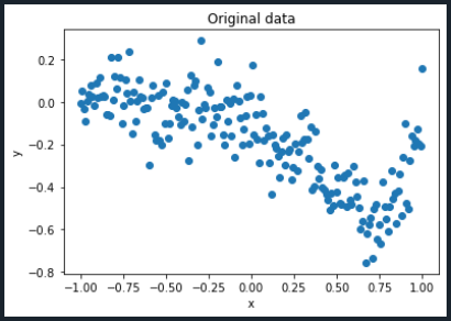
Said this, let's start coding! As you may remember from the previous tutorial, Python has a library called scikit-learn (please go to Python Machine Learning: Linear Regression (II)). The data used for this tutorial is similar to the one used in the Linear Regression tutorial, but now it has more x- and y- points

The first thing we should do is to import the text file containing the data (which has to be saved in the same folder as your Python script), then define the x- and y- values in order to plot them and have a graphical understanding of the data. Also, the x- array will be converted from 1D to 2D array using the function reshape(). (more details can be found in Python Machine Learning: Linear Regression (II)

#Importing libraries
import numpy as np
import matplotlib.pyplot as plt


#Importing text file
data = np.loadtxt('points.txt', skiprows=(2), dtype=float)
print(data)


#Setting x values
x = data[:,0]
print(x)


#Setting y values
y = data[:,1]
print(y)

#Converting the 1D-array into 2D-array
x_reshape = x.reshape(-1,1)
print(x_reshape)


#Plotting data
plt.plot(x,y,'o')
plt.title('Original data')
plt.xlabel('x')
plt.ylabel('y')
plt.show()

Now, it is time to define the degree of the polynomial. Remember that the higher the degree is, the more accurate the regression model will be. In order to do this, the Python library PolynomialFeatures is needed.

#Importing library
from sklearn.preprocessing import PolynomialFeatures


#Setting the polynomial degree
degree = PolynomialFeatures(degree = 5)

In order to fit the x-values to the defined polynomial degree, the function fit() is needed.

#Fitting the polynomial to the degree set previously
polynomial = degree.fit(x_reshape)

Now, like in the Linear Regression, it is necessary to build our Vandermonde matrix (please go to Python Machine Learning: Linear Regression (I) for more details).

#Creating our Vandermonde matrix according to the degree set previously
Vandermonde_matrix = degree.transform(x_reshape)
print(Vandermonde_matrix)

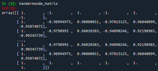
In the figure above, the first column is $x^0$, the second is $x^1$, and so on until the sixth column which is $x^5$ (5 is our defined polynomial degree). The number of rows will be equal to the number of $x$ points imported from the text file.

Now it is time to build the polynomial regression model. For this purpose, the library LinearRegression is needed. Yes, you read it correctly. Since Linear Regression is a particular case of Polynomial Regression as explained before, this library is needed.

#Creating the polynomial regression model
model = LinearRegression()

After having built the model, it necessary to fit the x- and y- values to the defined model. For this purpose, the library fit is needed. This means that the model will be trained getting the y-value for each x-value.

#Training the model (Fitting the Vandermonde matrix to the y-values)
train_model = model.fit(Vandermonde_matrix, y)

Now that the model is properly trained, it is time to use it! We will predict the corresponding y-values based on each x-value. For this, the function predict is needed.

#Getting the predicted y-values according to our x-Vandermonde matrix
y_predicted = train_model.predict(Vandermonde_matrix)

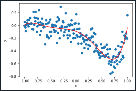
Finally, the last step is to plot. In order to have a better understanding of what was just done, the x- and y-values of the Polynomial Regression model and the initial x- and y-values will be plotted.

#Plotting the Polynomial Regression model
plt.plot(x,y,'o')
plt.plot(x,y_predicted,color='red')
plt.xlabel('x')
plt.ylabel('y')
plt.show()

The final Python code will look like the following:

#Importing libraries
import numpy as np
import matplotlib.pyplot as plt
from sklearn.preprocessing import PolynomialFeatures


#Importing text file
data = np.loadtxt('points.txt', skiprows=(2), dtype=float)
print(data)


#Setting x values
x = data[:,0]
print(x)


#Setting y values
y = data[:,1]
print(y)


#Converting the 1D-array into 2D-array
x_reshape = x.reshape(-1,1)
print(x_reshape)


#Plotting data
plt.plot(x,y,'o')
plt.title('Original data')
plt.xlabel('x')
plt.ylabel('y')
plt.show()


#Setting the polynomial degree
degree = PolynomialFeatures(degree = 5)


#Fitting the polynomial to the degree set previously
polynomial = degree.fit(x_reshape)


#Creating our Vandermonde matrix according to the degree set previously
Vandermonde_matrix = degree.transform(x_reshape)
print(Vandermonde_matrix)


#Creating the polynomial regression model
model = LinearRegression()


#Training the model (Fitting the Vandermonde matrix to the y-values)
train_model = model.fit(Vandermonde_matrix, y)


#Getting the predicted y-values according to our x-Vandermonde matrix
y_predicted = train_model.predict(Vandermonde_matrix)


#Plotting the Polynomial Regression model
plt.plot(x,y,'o')
plt.plot(x,y_predicted,color='red')
plt.xlabel('x')
plt.ylabel('y')
plt.show()

Congratulations! You just learnt the basics of regressions. Keep learning! To download the complete code and the text file containing the data used in this tutorial, please click here.