In the previous tutorial, you have learned how to build a linear regression using matrix multiplication (please go to Python Machine Learning: Linear Regression (I)). Now, in this tutorial, a Machine Learning Python library called scikit-learn will be used for this purpose.

Once we have imported the data from the text file, let's set our x- and y-values.

#Importing library
import numpy as np


#Importing text file
data = np.loadtxt('points.txt', skiprows=(2), dtype=float)
print(data)


#Setting x values
x = data[:,0]
print(x)


#Setting y values
y = data[:,1]
print(y)

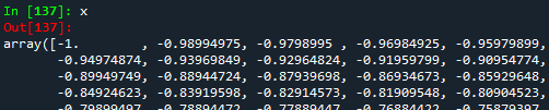
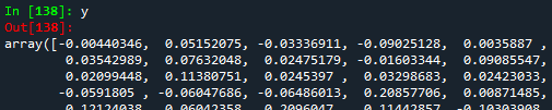
From the figure above (an extract of the whole data), we can notice that $x$ and $y$ are 1D arrays. If we want to work with the scikit-learn Machine Learning Python library, it is necessary to convert our 1D arrays into 2D. For this, the function reshape(-1,1).

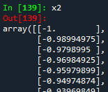
#Reshaping the array into a vector-column
x2 = data[:,0].reshape(-1,1)
print(x2)


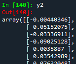
#Reshaping the array into a vector-column
y2 = data[:,1].reshape(-1,1)
print(y2)

Now, we are able to build our linear regression model using the LinearRegression module from the scikit-learn library. Do not forget to import the library.

#Importing library
from sklearn.linear_model import LinearRegression


#Building the linear regression model
linear_regression = LinearRegression()
linear_model = linear_regression.fit(x2,y2)

As explained in the previous tutorial, the linear relationship can be as \[y = c_{0} + c_{1}*x\], where $c_0$ is the intercept with the y-axis, and $c_1$ is the slope of the line. These two coefficients can be found easier and faster thanks to the function LinearRegression().fit(). In order to get both coefficients, the functions intercept_ and coef_ are needed.

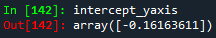
#Getting the intercept with y-axis
intercept_yaxis = linear_model.intercept_
print(intercept_yaxis)


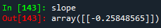
#Getting the coefficient
slope = linear_model.coef_
print(slope)

In contrast to the matrix multiplication approach where the coefficient matrix is an array of two elements, both elements are now got in two different arrays of one element each. If comparing both approaches, both intercept and slope should be exactly the same. The coefficient matrix from the previous tutorial was the following:

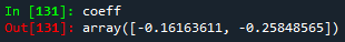
As seen from both pictures, we notice that both coefficients (intercept and slope) are exactly the same. This means we did a great job making the linear regression! Finally, let's establish the linear relationship and plot it.

#Importing library
import matplotlib.pyplot as plt


#Establishing the linear relationship
y_lineal2 = slope*x2 + intercept_yaxis
print(y_lineal2)


#Plotting


#Initially given x- and y-points
plt.scatter(x,y)


#Linear regression points
plt.plot(x2, y_lineal2, color='red')


#Naming the graph, x- and y-axis
plt.title('scikit-learn library')
plt.xlabel('x')
plt.ylabel('y')


plt.show()

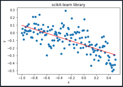
The plot we got in the previous tutorial was the following:

As seen from both graphics, we can say they are exactly the same! The final Python code will look like the following:

#Importing libraries
import numpy as np
from sklearn.linear_model import LinearRegression
import matplotlib.pyplot as plt


#Importing text file
data = np.loadtxt('points.txt', skiprows=(2), dtype=float)
print(data)


#Setting x values
x = data[:,0]
print(x)


#Setting y values
y = data[:,1]
print(y)


#Reshaping the array into a vector-column
x2 = data[:,0].reshape(-1,1)
print(x2)


#Reshaping the array into a vector-column
y2 = data[:,1].reshape(-1,1)
print(y2)


#Building the linear regression model
linear_regression = LinearRegression()
linear_model = linear_regression.fit(x2,y2)


#Getting the intercept with y-axis
intercept_yaxis = linear_model.intercept_
print(intercept_yaxis)


#Getting the coefficient
slope = linear_model.coef_
print(slope)


#Establishing the linear relationship
y_lineal2 = slope*x2 + intercept_yaxis
print(y_lineal2)


#Plotting


#Initially given x- and y-points
plt.scatter(x,y)


#Linear regression points
plt.plot(x2, y_lineal2, color='red')


#Naming the graph, x- and y-axis
plt.title('scikit-learn library')
plt.xlabel('x')
plt.ylabel('y')


plt.show()

Congratulations! You just made your first Machine Learning regression. In the next tutorial, polynomial regression will be explained. To download the complete code and the text file containing the data used in this tutorial, please click here.